loss functions: multiclass SVM and multinomial logistic regression

Loss functions quantify how good a W value is. It tells us how good our current classifier is and represents quantitatively our unhappiness with predictions on the training set. If it has a low value, that means our classifier is pretty good. If it has a higher value, then it's essentially telling us, "hey man, you need to change up your weights."

Because many people find it easier to optimize for higher values of something, sometimes we may consider the negative of the loss function. This is referred to as the reward function or utility function.

general expression for loss

Given a dataset of examples {(xᵢ, yᵢ)}ᵢ₌₁, where xi represents the image to be classified and yi, the index of the correct class, we can find the loss for a single example by using a function as shown: Lᵢ (F(xᵢ, W), yᵢ). Similarly, loss for the entire dataset can be expressed as the average of all the losses for all examples.

This varies based on the specific function you use to apply. We'll be exploring some of these below:

multiclass support vector machine (SVM) loss

The basic principle in multiclass SVM loss is that the score for the correct class must be much higher than all the other scores by a some fixed margin Δ, usually 1.

We start by defining a score function s = F(xi, W) = Wxᵢ + b.

For the j'th class, sⱼ = f(xi, W)ⱼ. This indicates the class score attained by the j'th class.

Now, multiclass SVM loss is computed by the following expression:



This expression looks pretty weird at first glance so let's break it down:

• (sⱼ- sᵧᵢ + Δ) → this part indicates the difference between the scores of each class and that of the correct class. The margin value is added to it.
• The max function is a function that returns the highest value from a set of values. Here, we want to return value 0 as much as possible (as that would imply low loss values), which means that we are trying to get (sⱼ- sᵧᵢ + Δ) <= 0. For 0 loss, the highest score among all the incorrect classes to be at a certain margin from the score for the correct class.
• In other words, the correct class must have a score at least Δ greater than the score assigned to all the incorrect categories.
• The loss for each category is summated across all of the incorrect categories (thus the j != yᵢ below the summation symbol) to give us the final value.

The threshold at zero max(0,-) is often called the hinge loss. It can be illustrated with this graph:



Some prefer using squared hinge loss SVM (aka L2-SVM), which uses the form max(0, -)² which punishes violated margins more severely. You may choose between the 2 depending on your dataset.

A randomly initialized model would spit out the same scores for all categories. In that case, our loss would approximately be (N-1)Δ, where N is the number of classes/categories.

the problem: uncertainty in the model

Now there's one tiny problem with our loss function. Let's say we tried tweaking around and finetuning the values of our weights and finally found one that gives us the average loss L = 0. Woohoo!

But then you experiment and try 2W, and.... it also gives L = 0? And then 3W, 4W and so on until you finally realize that all of them give you the same loss. This introduces uncertainties to your model and you're left confused as to which set of weights to select, seeing as they all produce identical results.

why does this happen?

If one set of weights correctly classifies all examples, then any multiple of these weights λW (where λ > 1) will also result in zero loss. Why is that?

Keep in mind that the score is a linear function of the weights and pixels. Thus, multiplying all elements of W by a common factor simply scales the scores achieved by the model, without changing their relative differences. All it does is essentially "stretch" the distances between the scores achieved by the model.

introducing regularization

The problem outlined earlier leads us to modify our loss expression a little bit. In order to express preferences between classifiers, we introduce a regularization term R(W) in the loss function, given by:



Here, we sum up all squared elements of W.

By including this term, we get a revised expression, consisting of 2 components; data loss (the average L over all the examples) and regularization loss. Thus, the final multiclass SVM loss expression becomes:



The λ term introduced is a hyperparameter known as regularization strength. This value is usually determined by cross-validation methods.

In L2 generalization, we generally steer clear from larger weights, penalizing them with the regularization loss value. Here, we consider the squared value of the weights in the regularization term R(W) as shown previously. The classifier is encouraged to take into account all input dimensions to small amounts by using smaller and more diffuse weights rather than considering only a few input dimensions severely.

On the other hand, L1 regularization tells the model to put all the weights to a single feature. In the regularization term, instead of taking the squared value of the weights, we consider the absolute value. This works better for feature selection when we have a large number of features.

multinomial logistic regression (cross entropy loss)

Another loss function that is commonly used is known as multinomial logistic regression. It takes up a different approach to classifiers, interpreting the raw scores given by the classifier as probabilities.

There are 4 steps to computing loss via this method:

1. Take raw scores predicted by the classifier for each category (found by the score function). These scores are referred to as unnormalized log probabilities or logits.
2. Run logits through exponential function to obtain unnormalized probabilities. This makes the values of the probabilities positive.
3. Calculate the sum of unnormalized probabilities. Divide each probability with the sum to get what is called normalized probabilities. This is done to ensure that the probabilities add up to 1.
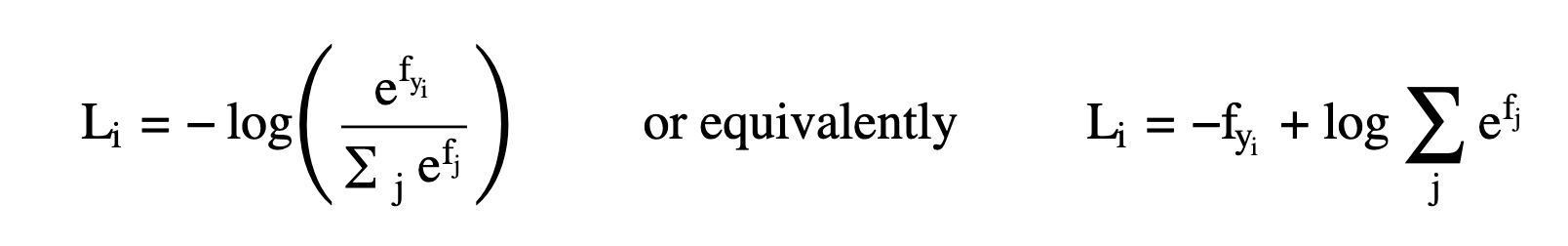
4. Now, we actually assess our model! We apply a negative logarithm on the normalized probability of each image in our training set, take average and obtain overall loss.

The first 3 steps can be mathematically expressed as:



This is known as the "softmax function". This function takes in the raw scores and spits out a valid probability distribution. This image by Kiprono Elijah Koech on Towards Data Science sums it up perfectly:



All in all, loss is calculated using the below expression:



Two very popular methods to compare probabilities are:

• The Kullback-Leibler Divergence
• Cross entropy

Unlike multiclass SVM loss, it is much harder to achieve 0 loss in this scenario. This is because the ideal probability distribution that would result in 0 loss is one where everything but the correct class has a normalized probability of 0. This is virtually impossible to achieve.

If the model has been randomly initialized, then the loss is likely to be -log(1/N) = logN. Thus, for CIFAR10 dataset, random initialization would result in L = log10 = 2.3.