A tutorial problem that really helped me get an intuition for content from 5A!
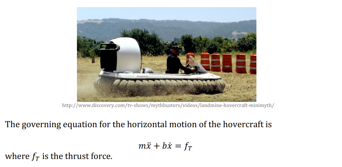
Consider this hovercraft:
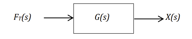
Naively, we can represent the hovercraft through a simple block diagram:
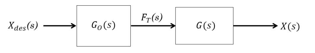
To get a certain
X_\text{des}(s) Xdes(s) , we can solve for a G_O(s) GO(s) block to get F_T(s) FT(s) :The solution is straightforward:
X = G_O G X_\text{des} \\
\implies G_O = \frac{1}{G} = ms^2 + bs
X=GOGXdes⟹GO=G1=ms2+bs The problem with this control system -- known as "open loop" control because there is no feedback cycle -- is that it has no resistance to error.
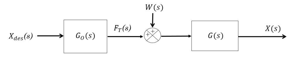
Consider an unaccounted-for wind force
acting on the system:Now the behavior of the entire system is:
\begin{align*}
X &= G(W + F_T) \\
&= G(W + G_O X_\text{des}) \\
&= GW + G G_O X_\text{des} \\
&= GW + X_\text{des} \\
\end{align*}
X=G(W+FT)=G(W+GOXdes)=GW+GGOXdes=GW+Xdes Consider the final value of this system using the final value theorem for some step input
W(s) = \frac{W_\text{in}}{s} W(s)=sWin :\begin{align*}
\lim_{t\to\infty} x(t) &= \lim_{s\to 0} s(X(s)) \\
&= \lim_{s\to 0} s(GW + X_\text{des}(s)) \\
&= \lim_{s\to 0} s\bigg(\frac{1}{ms^2 + bs} \frac{W_\text{in}}{s} + X_\text{des}(s)\bigg) \\
&= \lim_{s\to 0} \frac{1}{ms^2 + bs} W_\text{in} + X_\text{des}(s)s \\
\end{align*}
t→∞limx(t)=s→0lims(X(s))=s→0lims(GW+Xdes(s))=s→0lims(ms2+bs1sWin+Xdes(s))=s→0limms2+bs1Win+Xdes(s)s Remember that
X_\text{des}(s) Xdes(s) is not itself a constant. If x_\text{des}(t) xdes(t) is a constant, X_\text{des}(s) Xdes(s) is the Laplace transform of the constant, with the value \frac{x_\text{const}}{s} sxconst . In the above limit, then, X_\text{des}(s)s = \frac{x_\text{const}}{s}s = x_\text{const} Xdes(s)s=sxconsts=xconst -- absent wind, the final value is just the desired value, as expected.The first term, on the other hand, has a denominator that goes to 0. Unless
W_\text{in} = 0 Win=0 , the entire term will thus blow up to infinity.And that makes sense! Wind error is entirely uncorrected for, so the hovercraft will drift farther and farther off of its desired path over time.
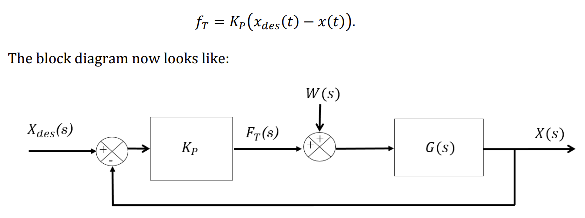
To fix this, let's replace open loop control with proportional control. That is, we'll swap out the
block for a block and a node for calculating error:Now the system behavior can be characterized by the following equation:
\begin{align*}
X &= G(W + F_T) \\
&= G(W + K_P (X_\text{des} - X)) \\
\implies X &= \frac{G}{1+K_P G}W + \frac{K_P G}{1+K_P G}X_\text{des} \\
\end{align*}
X⟹X=G(W+FT)=G(W+KP(Xdes−X))=1+KPGGW+1+KPGKPGXdes Once again we have a term for wind and one for control.
Let's take a look at the final value of the control term:
\begin{align*}
x_\text{final, control} &= \lim_{s\to0} s \frac{K_P G}{1+K_P G}X_\text{des} \\
&= \lim_{s\to0} s \frac{K_P \frac{1}{ms^2 + bs}}{1 + K_P \frac{1}{ms^2 + bs}} X_\text{des} \\
&= \lim_{s\to0} s \frac{K_P}{ms^2 + bs + K_P} X_\text{des} \\
\end{align*}
xfinal, control=s→0lims1+KPGKPGXdes=s→0lims1+KPms2+bs1KPms2+bs1Xdes=s→0limsms2+bs+KPKPXdes For a constant
X_\text{des} = \frac{x_\text{const}}{s} Xdes=sxconst , x_\text{final, control} = \frac{K_P}{K_P} X_\text{des} = X_\text{des} xfinal, control=KPKPXdes=Xdes , as expected. We can also note that this system has a second-order transfer function: for a step response X_\text{des} Xdes , we can expect an output that rises exponentially to the steady state value, possibly overshooting depending on .Now let's look at wind for step input
W(s) = \frac{w_\text{in}}{s} W(s)=swin :\begin{align*}
x_\text{final, wind} &= \lim_{s\to0} s \frac{G}{1+K_P G}W \\
&= \lim_{s\to0} s \frac{\frac{1}{ms^2 + bs}}{1 + K_P \frac{1}{ms^2 + bs}} \frac{w_\text{in}}{s} \\
&= \lim_{s\to0} \frac{w_\text{in}}{ms^2 + bs + K_P} \\
&= \frac{w_\text{in}}{K_P}
\end{align*}
xfinal, wind=s→0lims1+KPGGW=s→0lims1+KPms2+bs1ms2+bs1swin=s→0limms2+bs+KPwin=KPwin We find that there is still an error, but the error is finite now, and smaller the higher
is. This error also has a second-order step response.A nice example of proportional control and the math behind it!

 Samson Zhang